The following scenarios showcase the use of the group_aggregate function in the real world. We provide them to demonstrate to you how the function works, and the scenarios where it proved useful.
- Scenario 1: Supplier tendering by job
- Scenario 2: Average rates of exchange
- Scenario 3: Average period value for semi-additive numbers I
- Scenario 4: Average period value for semi-additive numbers II
Best practices for flexible aggregations
The group_aggregate function enables you to calculate a result at a specific aggregation level, and then returns it at a different aggregation level. For this reaggregation result to return correctly, follow these syntax guidelines:
-
Wrap
group_aggregatein an aggregate function, such assumoraverage -
The wrapping function must be the immediate preceding function, such as
sum(group_aggregate(...)) -
Do not use with conditional operators. For example, the following expression does not reaggregate the data because the
ifprecedesgroup_aggregate:(if(group_aggregate(...)))
Scenario 1: Supplier tendering by job
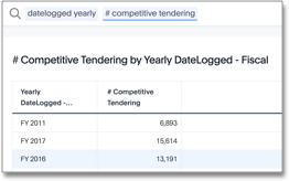
We have a fact table at a job or supplier tender response aggregation level. There are many rows for each job, where each row is a single row from a supplier. A competitive tender is a situation when multiple suppliers bid on the same job.
Our objective is to determine what percentage of jobs had more than 1 supplier response. We want to see high numbers, which indicate that many suppliers bid on the job, so we can select the best response.
Valid solution
A valid query that meets our objective may look something like this:
sum(group_aggregate(if(sum(# trades tendered ) > 1) then 1 else 0,
                    query_groups() + {claimid, packageid},
                    query_filters()))

Resolution
The
sum ( # trades tendered )function aggregates to these attributes:-
{claimid, packageid}The job-level identifier
-
query_groups( )Adds any additional columns in the search to this aggregation. Here, this is the
dateloggedcolumn at the yearly level. -
query_filters ( )Applies any filters entered in the search. Here, there are no filters.
-
For each row in this virtual table, the conditional
if() then elsefunction applies. So, if the sum of tendered responses is greater than 1, then the result returns 1, or else it returns 0.The outer function,
sum(), reaggregates the final output as a single row for eachdateloggedyearly value.- This reaggregation is possible because the conditional statement is inside the
group_aggregatefunction. - Rather than return a row for each
{claimid,packageid}, the function returns a single row fordatelogged yearly. - The default aggregation setting does not reaggregate the result set.
- This reaggregation is possible because the conditional statement is inside the
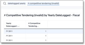
Non-Aggregated Result
We include the following result to provide contrast to an example where ThoughtSpot does not reaggregate the result set. Reaggregation requires the aggregate function, sum, to precede the group_aggregate function.
In the following scenario, the next statement is the conditional if clause. Because of this, the overall expression does not reaggregate. The returned result is a row for each {claimid,packageid}.
sum(if(group_aggregate (sum (# trades tendered),
                              query_groups() + {claimid, packageid},
                              query_filters ( ) )>1) then 1 else 0)
Scenario 2: Average rates of exchange
The Average rate of exchange calculates for the selected period. These average rates provide a mechanism to hedge the value of loans against price fluctuations in the selected period. We apply the average rate after the aggregation.
The pseudo-logic that governs the value of loans is sum(loans) * average(rate).
The data model has two tables: a primary fact table, and a dimension table for rates.
- The
loanscolumn is from the primary fact table. - The
ratecolumn is from theratestable.
These tables are at different levels of aggregation:
- The primary fact table uses a lower level of aggregation, on
product,department, orcustomer. - The
ratesdimension table use a higher level of aggregation, ondaily,transaction currency, orreporting currency.
The two tables are joined through a relationship join on date and transaction currency.
To simplify the scenario, we only use a single reporting currency. The join ensures that a single rate value returns each day for each transaction currency.
Valid solution
A valid query that meets our objective may look something like this:
sum(group_aggregate (sum(loans)*average (rate),
                     query_groups () + {transaction_currency},
                     query_filters () ))
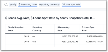
The following search and resulting response returns the dollar value for each year, for each target reporting currency. Note that the dataset contains both euro (€) and US dollars ($). The $ Loans Avg. Rate calculates the average rate of exchange for the entire period. The $ Loans Spot Rate applies the rate of exchange on the day of the transaction.

Resolution
The
sum(loans)function aggregates to these attributes:-
{transaction_currency}andquery_groups()Add additional search columns to this aggregation. Here, this at the level of
reporting currencyandyear. -
query_filters( )Applies any filters entered in the search. Here, there are no filters.
-
Similarly, the
average(rate)function aggregates to these attributes:-
{transaction_currency}andquery_groups()Add additional search columns to this aggregation. Here, this at the level of
reporting currencyandyear. -
query_filters( )Applies any filters entered in the search. Here, there are no filters.
-
For each row in this virtual table, the exchange rate applies to the sum of loans:
sum(loans) * average(rate).The outer
sum()function reaggregates the final output as a single row for each yearly reporting currency value.Note that the default aggregation setting does not reaggregate the result set.
Non-Aggregated Result
We include the following result to provide contrast to an example where ThoughtSpot does not reaggregate the result set. Reaggregation requires the aggregate function, sum, to precede the group_aggregate function.
In the following scenario, the formula assumes that the default aggregation applies. Here, the result returns 1 row for each transaction currency.
group_aggregate (sum(loans )*average (rate ),
                 query_groups() + {transaction_currency},
                 query_filters())

Scenario 3: Average period value for semi-additive numbers I
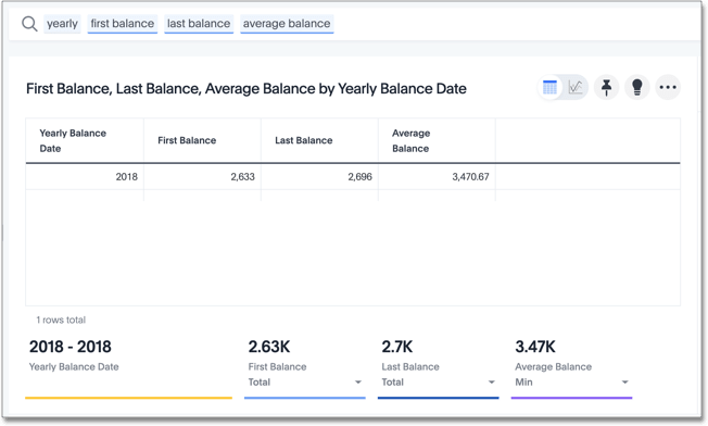
Semi-additive numbers may be aggregated across some, but not all, dimensions. They commonly apply to specific time positions. In this scenario, we have daily position values for home loans, and therefore cannot aggregate on the date dimension.
Valid solution
A valid query that meets our objective may look something like this:
average(group_aggregate(sum(loan balance),
                        query_groups() + {date(balance date)},
                        query_filters()))

Resolution
The
sum(loan balance)function aggregates to the following attributes:-
{date(balance date)}andquery_groups()Add additional search columns to this aggregation. Here, this at the
yearlylevel. -
query_filters ( )Applies any filters entered in the search. Here, there are no filters.
-
The
sum(loan balance)function returns a result for each row in this virtual table.The outer
average()function reaggregates the final output as a single row for eachyearvalue.
Scenario 4: Average period value for semi-additive numbers II
Semi-additive numbers may be aggregated across some, but not all, dimensions. They commonly apply to specific time positions. In this scenario, we have daily position values for home loans, and therefore cannot aggregate on the date dimension.
Here, we consider a somewhat different situation than in Scenario 3. In some financial circumstances, the average daily balance has to be calculated, even if the balance does not exist. For example, if a banking account was opened on the 15th of June, business requirements have to consider all the days in the same month, starting with the 1st of June. Importantly, we cannot add these ‘missing’ data rows to the data set; note that the solution used in Scenario 3 returns an average only for the period that has data, such as June 15th to 30th, not for the entire month of June. The challenge is to ensure that in the daily average formula, the denominator returns the total days in the selected period, not just the days that have transactions:
sum(loans) / sum(days_in_period)To solve for this, consider the data model:
- The fact table
transactionsreports the daily position for each account, and uses aloancolumn. - The dimension table
datetracks information for each date, starting with the very first transaction, all the way through the most recent transaction. This table includes the expecteddatecolumn, anddays_in_periodcolumn that has a value of 1 in each row. - Worksheets use the
datecolumn with keywords such as weekly, monthly, yearly to change the selected period. - When users run a search with the monthly keyword, the denominator must reflect the number of days in each month.
Valid solution
A valid query that meets our objective may look something like this:
The following code in the denominator definition returns the total number of days for the period, regardless whether there are transactions, or what filters apply:
group_aggregate (sum(days_in_period),{Date},{})
Resolution
-
The
sum(days_in_period)function aggregates to:{Date}No other search columns appear.
{}We require the entire period, so there are no filters.
Note that the
datekeywords yearly, quarterly, monthly, and weekly apply because we use the same column in both the search and the aggregation function. So, the function will result in the following output when it runs with the yearly keyword in search:Year Result 2016 366 2017 365 2018 365 2019 365 2020 366 -
This data is not reaggregated because we want to return the result at the appropriate
datelevel.
Alternate Solution
To return only the number of days that have existing transactions, use the following code in the denominator:
sum(days_in_period)